Documentation CRN-Method with LSDTopoTools
Get DEM at https://opentopography.org/, select your area and select under 'Global & Regional DEM' the 'Shuttle Radar Topography Mission (SRTM) Global SRTM GL3'
Step 1) Start LSDTopoTools and other preparation
Start the docker container and then PowerShell
Start LSDTopoTools with:
# docker run --rm -it -v C:/LSDTopoTools:/LSDTopoTools lsdtopotools/lsdtt_pcl_docker
Then start docker in PowerShell with:
# Start_LSDTT.sh
If you don’t have the Example data, download it with:
# Get_LSDTT_example_data.sh
These command lines will update the program and look for new files etc.:
# sh build.sh
# cd..
# sh lsdtt2_terminal.sh
After the process is finished navigate to your directory in which your data is located or in which you want to operate.
For navigation use cd..your_folder_name (to access subdirectories) or cd.. to return in the folder above.
If you used cd you are in the uppermost directory level. Use cd/LSDTopoTools to find the directory again.
Step 2) Create a folder inside the LSDTopoTools directory
First, a folder in the subdirectory of LSDTopoTools must be created. Use a name without special characters or spaces (here sample17).
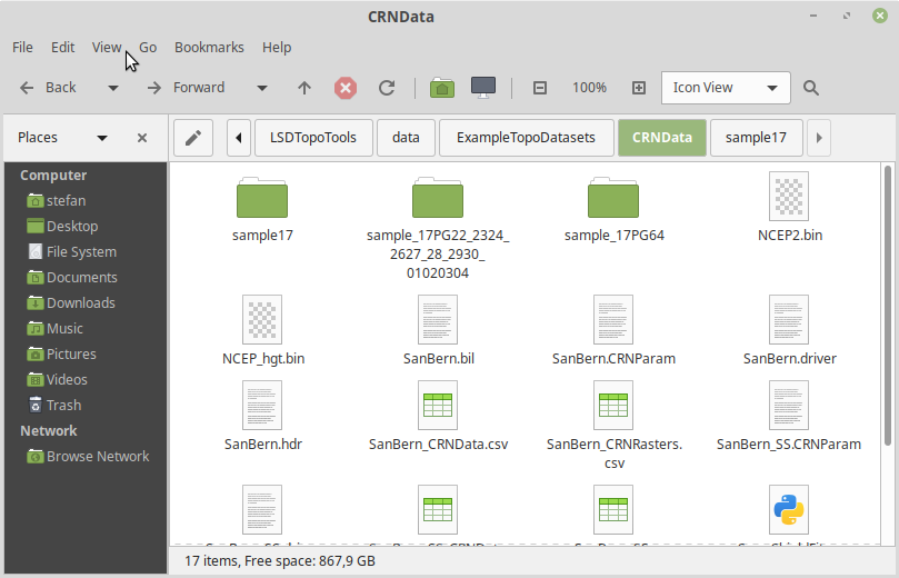
Figure 1: For this example, sample 17 was created
In the example folder following files should be present:
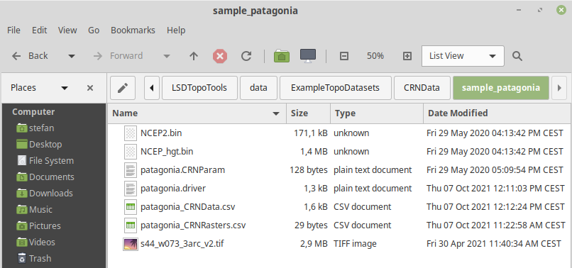
Figure 2: necessary files for the first step in the CRN-computation method
The CRNparam-file contains your settings, the .driver-file contains the command lines (see later), the .CRNData.csv-file has the information of your sample points (name, latitude, longitude, type of nuclide, nuclide concentration, uncertainty, and standardization), NCEP_hgt.bin & NCEP2.bin which are atmospheric datafiles, CRNRaster.csv which contents the file path to all your data (see later) and the DEM.tif
Troubleshoot: If your DEM is too big the computation is ‘killed’ -> you have to clip the .tif (your DEM) with QGIS (insert the CRNData.csv and clip the .tif only where the sample locations are; don’t cut the basins respectively leave enough space)
For a CRNData.csv template look at LSDTopoTools/data/ ExampleDataSamples/CRNData/SanBern
Step 3) create the -bil-file from your DEM
First, you have to look up in which zone and hemisphere your DEM/basin is located.
Then create .bil file with the following code:
# gdalwarp -t_srs '+proj=utm +zone=18 +south +datum=WGS84' -of ENVI name_of_your_source DEM.tif name_of_your_new_DEM.bil
All data files have the given name you have chosen for ‘name_of_your_new_DEM’ in the code.
Here the DEM is called patagonia.bil
The UTM zone and the hemisphere is for this step mandatory. The code creates new data (.bil, .bil.aux.xml, .hdr) in the same folder where all the other data is located.
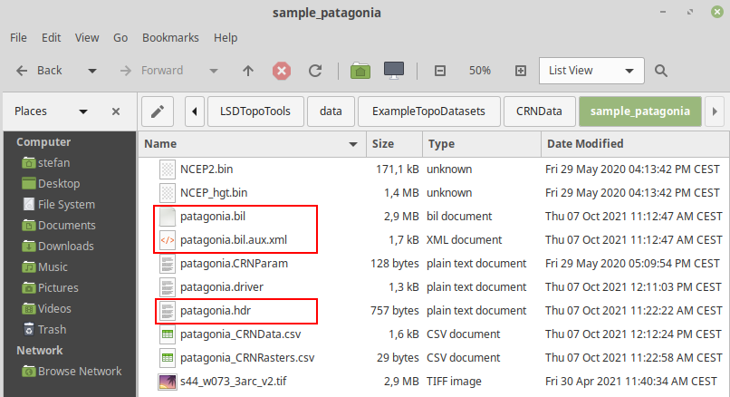
Figure 3: new created .bil & .hdr files
Step 4) prepare the driver file, CRNParam, CRNRaster.csv, CRNData.csv, and compute the first step in the driver file
The necessary data inside the folder (before any computation is taking place) besides the created DEM of your area should be the driver file, the CRNParam, CRNRasters, and CRNData.
Caution: The driver-file and the CRNParam must have the same name as your bil-file (here: patagonia.driver and patagonia.CRNParam)
For a driver-file template look at LSDTopoTools/data/ ExampleDataSamples/CRNData/SanBern or in the attatchment of this document.
Open the driver file and change the read fname at the top to the name of your .bil file and all other commands and cosmo parameter prefixes in steps 1 to 4.
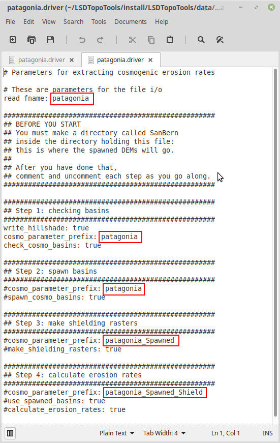
Figure 4: driver-file with changes prefixes
Change the directory in the CRNRaster.csv to:
./your_bil_file_name
In this example it would be:
./patagonia (should be the same name as in the .bil file or all other files!)
Now, prepare your CRNData.csv file with the name of your samples, the method (10Be), the standard, and the concentration respectively the error of the concentrations. Additional data like shielding can be also included. Save the document as a .csv file.
For more info on how to write the CRNData.csv go to:
https://lsdtopotools.github.io/LSDTT_documentation/LSDTT_BasinwideCRN.html
under 3.3.2 The cosmogenic data file
Now the first computation can be carried out.
You can find a video on how the computation is performed here: https://www.youtube.com/watch?v=8nIIcxNzrUY&list=PLVwZ3VSC-2RTQmVvUSbBwdHsLxTNJ8IDK&index=6&t=110s
Uncomment successively your commands in the driver file. So first uncomment step 1 then run the driver with:
# lsdtt-cosmo-tool patagonia.driver
You can adjust your parameters in the CRNparam file if you need other results.
NOTE: If the program shows the message ‘killed’ your DEM.bil is to big (then you should clip it). The first computation could last a while!
New data is created. Your folder should contain files with these endings:
_hs.bil, _hs.hdr, CRNParamReport, AllBasins.info.csv, BasinKey.csv, AllBasins.hdr, AllBasins.bil, CN.csv
Step 5) second computation in the driver file
Comment step 1 in driver file, uncomment step 2. This step spawns all the basins in your DEM. First, you have to create a new folder in which the new basin files are saved (NOTE: this folder has to be created once. A re-creation during a rerun with the added snowraster (see below: snow shielding computation) is not necessary). This should have the same prefix as the data prefix (here: patagonia):
# mkdir patagonia
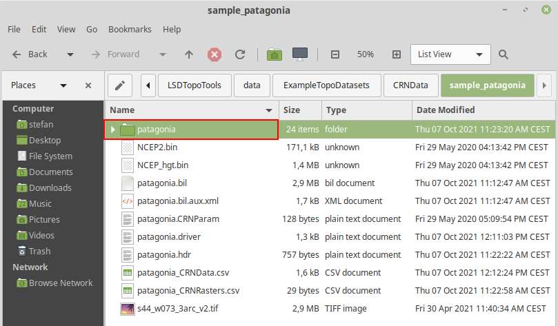
Figure 5: newly created folder
You can check in LSDTopoTools with
# ls
if it is created:
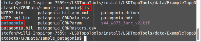
Figure 6: newly created folder in LSDTopoTools
Before you run the computation check if the cosmo parameter prefix is Chile_sample (see figure 4).
Now the driver file can be run again with:
# lsdtt-cosmo-tool patagonia.driver
In the folder, the new basins will be created. .bil and .hdr-files for each DEM will be created:
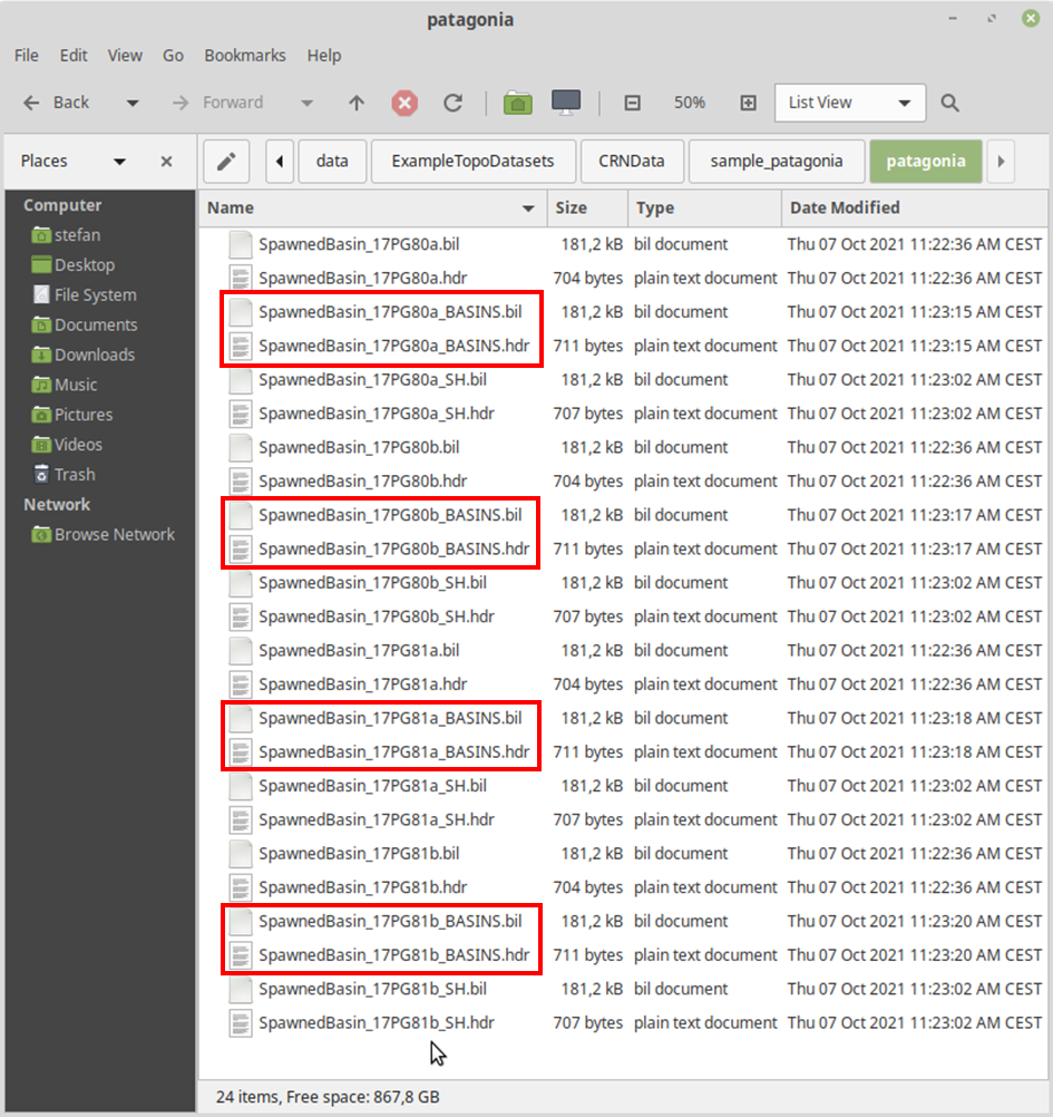
Figure 7: newly spawned basins in the created folder
Step 6) third step in driver file (Shielding is created)
Before you run the computation check if the cosmo parameter prefix is correct. (here: patagonia_Spawned, see figure 4).
Then run the driver with:
# lsdtt-cosmo-tool patagonia.driver
This computation step creates new data in your general directory. CRNParamReport, CRNParam, Spawned_Shield_CRNData.csv, and Spawned_shield_CRNRasters.csv should be created (see figure 8).
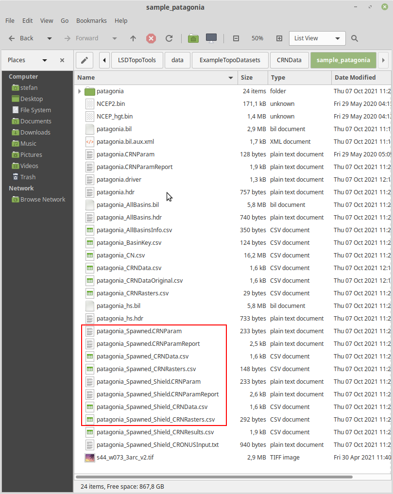
Figure 8: created shielding files with the third step of the driver file (NOTE: This step creates no/wrong snow shielding unless you created a snowraster (see below: snow shielding computation)) and rerun this step of the driver file.
Furthermore, this should create files with SH in the created subdirectory from the step prior (see figure 9). These files have the shielding data for each basin.
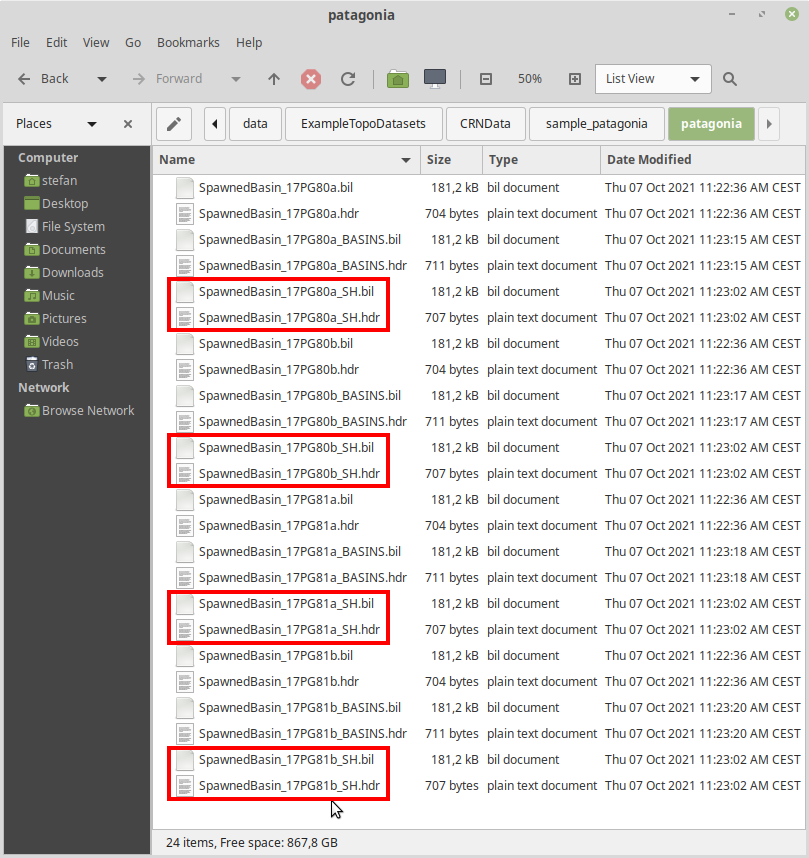
Figure 9: new created shielding files in the subdirectory
Step 7) fourth step in the driver file (creates the erosion rates and the final result.csv files)
In the last computation step, you get your final data with the results. (NOTE: This step creates the erosion rates with no/wrong snow shielding unless you created a snowraster (see below: snow shielding computation)) and rerun this step of the driver file.
For a description for every single column look here:
https://lsdtopotools.github.io/LSDTT_documentation/LSDTT_BasinwideCRN.html
Chapter 6.3: The output files
Before you run the computation check if the cosmo parameter prefix is correct (here: patagonia_Spawned_Shield, see figure 4).
Then run the driver with:
# lsdtt-cosmo-tool patagonia.driver
This last computation creates again a ParamReport and the CRONUSInput.txt as well the final results Spawned_ShieldsCRNResluts.csv
The ParamReport shows the input of parameters like shielding and the values of the used parameters at the beginning. If results aren’t satisfying change the parameter in the param file or in the driver file and redo all the steps above. For more information visit:
https://lsdtopotools.github.io/LSDTT_documentation/LSDTT_BasinwideCRN.html
Documentation CRN-Method with LSDTopoTools - Snow Shielding computation
Before you do any snow shielding computation, you have to add the name of the snow shielding raster to the CRNRaster.csv.
For example: If your glacier raster is called raster_patagonia.bil add it without the '.bil'. Your CRNRasters.csv should look like this: ./patagonia ./raster_patagonia
NOTE: add ./patagonia and ./raster_patagonia in two separate columns in the CRNRasters.csv
Creation of the glacier shielding raster:
First use a shapefile of the glacier data (e.g. GLIMS glacier polygons) and copy it in your directory.
Then create the DEM (for command see Step 3) or use the DEM from before (e.g. patagonia.bil).
Following use gdalinfo on the DEM -> copy the corner coordinates (upper left, lower left, ...) and the Pixel size (see figure 10).
At last run: gdal_rasterize -a_nodata -9999 –burn 9000 –of ENVI -a_srs '+proj=utm +zone=18 +south +datum=WGS84' -te <xmin> <ymin> <xmax> <ymax> -tr <xres> <yres> -ot Int16 GLIMSshapefile.shp glacier_raster.bil to create the glacier raster (see figure 11).
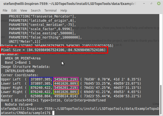
Figure 10: Information of the created DEM. <xmin(blue)> <ymin(orange)> <xmax(green)> <ymax(purple)> <xres> <yres> (red)
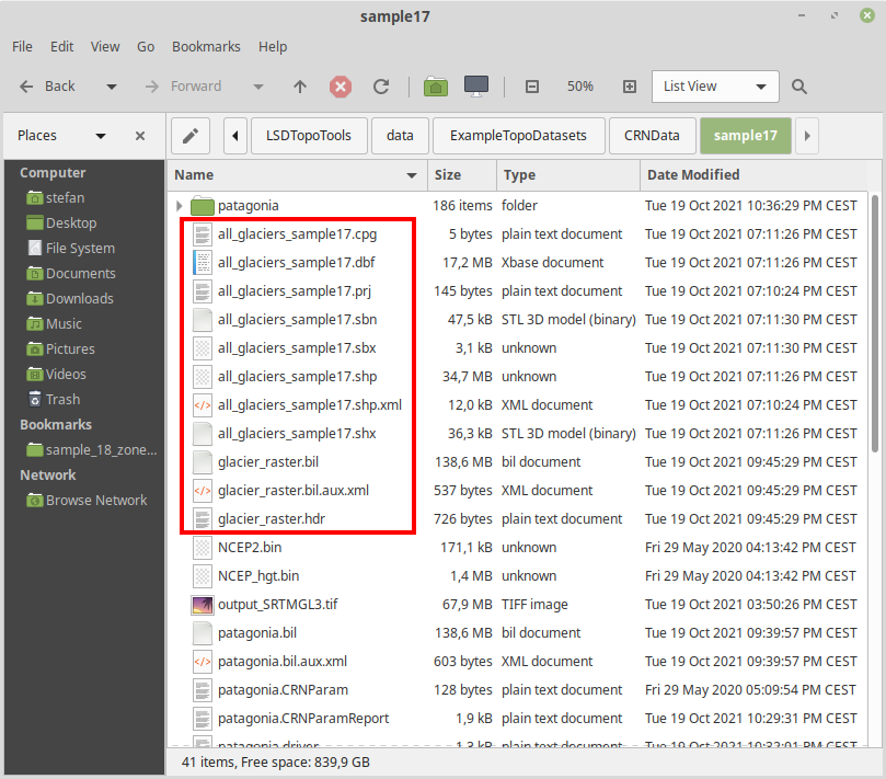
Figure 11: the created glacier_raster and glacier shapefile
NOTE: The name of your '.bil' snowraster (e.g. snowraster_patagonia.bil) has to be the same as added in the CRNRasters.csv
NOTE: The DEM and the shapefiles of GLIMS have to be in the same projection system.
IMPORTANT: If you don’t get correct shielding values check the glacer_raster in ArcGIS or QGIS. If the values aren’t from 0 to 9000 for the glacer_raster the computation didn’t work correctly. For this don’t change the projection from the DEM and glacier shapefile in LSDTopoTools, instead use the projection tool in ArcGIS and project the DEM and glacier shapefile into the same projection. Then use your projected DEM and glacier shapefile and change the commands for creating the DEM.bil and glacer_raster.bil in LSDTopoTool as follows:
gdal_translate -of ENVI name_of_your_source_DEM.tif name_of_your_new_DEM.bil
gdal_rasterize -a_nodata -9999 -burn 9000 -of ENVI -te xmin ymin xmax ymax -tr xres yre -ot Int16 GLIMSshapefile.shp glacier_raster.bil
Now you can rerun the third and fourth steps in the driver file described above.
NOTE: If you rerun all steps of the driver file (for example you had your snowraster from the beginning) then an error message at the second driver computation can occur. To solve this problem delete the ./snowraster_patagonia in the CRNRaster.csv and rerun this step. Insert ./snowraster_patagonia for the third and fourth driver computation.
Attachment
Driver for the computation:
Parameters for extracting cosmogenic erosion rates
# These are parameters for the file i/o
read fname: patagonia
####################################################
## BEFORE YOU START
## You must make a directory called patagonia
## inside the directory holding this file:
## this is where the spawned DEMs will go.
##
## After you have done that,
## comment and uncomment each step as you go along.
####################################################
####################################################
## Step 1: checking basins
####################################################
write_hillshade: true
cosmo_parameter_prefix: patagonia
check_cosmo_basins: true
####################################################
## Step 2: spawn basins
####################################################
#cosmo_parameter_prefix: patagonia
#spawn_cosmo_basins: true
####################################################
## Step 3: make shielding rasters
####################################################
#cosmo_parameter_prefix: patagonia_Spawned
#make_shielding_rasters: true
####################################################
## Step 4: calculate erosion rates
####################################################
#cosmo_parameter_prefix: patagonia_Spawned_Shield
#use_spawned_basins: true
#calculate_erosion_rates: true
Sources:
[1] https://lsdtopotools.github.io/LSDTT_documentation/index.html (last accessed 17.11.2021)
[2] Mudd, S. M., Harel, M.-A., Hurst, M. D., Grieve, S. W. D., and Marrero, S. M.:
The CAIRN method: automated, reproducible calculation of catchment-averaged denudation
rates from cosmogenic nuclide concentrations, Earth Surf. Dynam., 4, 655-674,
doi:10.5194/esurf-4-655-2016, 2016.