---

 

Tutorial 1: Learn how to display, manage and analyze elevation data in ArcMap.

 

OBJECTIVE:

The overall objective of this exercise is to give you an overview of ArcGIS, basic GIS operations and tools for digital terrain analysis.  

 

Relative Paths – It is best to set the .mxd’s data source to relative paths so that ArcGIS can find the data referenced in an .mxd if the project and its data are moved to a different drive or folder. To do so:

• click on the Customize menu
• click on ArcMap Options
• Go to General
• Check the box next to “Make relative paths the default for new map documents”
• Click OK.

Note! Save your ArcMap (.mxd file) regularly throughout this exercise.

 

 

1. Exploring and Visualizing the DEM

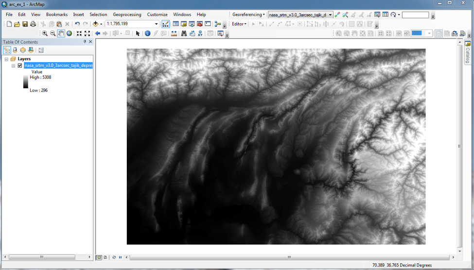
1. Start ArcMAP from Start->programs->ArcGIS menu on your windows computer. Begin with a new, blank document in ArcMap. Choose File->Save and navigate to the folder on your USB stick you want to save it to and name the file “arc1_ex_XX” where XX is your initials. Download the elevation data file nasa_srtm_v3.0_3arcsec_tajik_depression.tif.zip, safe it to the same folder and unzip the file. Then, click on Add data button and navigate to your folder and click on Add. Your DEM will be displayed as a gray scale image with the lowest values black and the highest values white. It should look like this:

 

First, create a raster attribute table. Open Toolbox, go to Data Management Tool/Raster/Raster Properties/Build Raster Attribute Table.

You can change this setting in the Layer Properties dialog. To do this, right click on your DEM file in the Table of Contents. Choose Properties from the bottom of the menu, and go to the Symbology dialog. The default setting for grid data is Stretched. Try several of the color ramps to try to improve the visualization of the terrain. Pick one you think will work better than the greyscale default. Click Apply and move the properties dialog aside so you can see what the DEM looks like in the selected map.

Then, click on the Show item Classified. This will divide the values (elevations) of the DEM into a number of groups or bins, each of which can be assigned a different color. The default is for 5 bins. Select the Color Ramp you used before. Click Apply. It may not look good with only 5 classes! Click the Classify button in the upper right of the dialog. The histogram of the distribution of the elevation values is the central feature of the Classification dialog. Make sure the number of classes is 5 and that the Method is Equal Interval. Click OK, and then Apply and look at the DEM as before. If you are not happy with the results, try increasing the number of classes and see what happens.   

Review what you have done:

a. Which symbolizations of your DEM do you prefer? Ramp or # of classes? Click OK when you are happy with what you have.

b. Click on the View tab in the main navigation bar. Select Layout View. Then click on Insert in the main navigation bar. Using this menu, insert a title, legend and scale bar for your map. To insert Grids, click on View and select Data Frame Properties. Click on Grids, and create a new grid (Graticule). Click OK. Add your name (required) to the map (Insert->Text). Then go to File->Export Map and save your map as tiff. You will include this map in your final PDF file.

c. Why do you like to display your data this way? Think about what you would like to communicate to the viewer?

 

2. Return to View->Data View. Right click on Layers, and select Properties. Open the Coordinate System tab, and check that the Current coordinate system matches that of the DEM file. Click OK. In the Table of Contents, right click on your DEM file and choose Properties. Answer the following questions:

a. What is the current coordinate system?

b. Number of cells on the x- and y-axis?

c. Total number of cells in the grid?

d. What is the cell size in x and in y?

e. What are the linear units?

Close the Layer Properties dialog. Right click on your DEM file again.

 f. Is there an attribute table? Is the grid integer numbers or floating point (real numbers)?

 

3.  Before we move to the next section, you need to know about the z-factor. The z-factor is a conversion factor that adjusts the units of measure for the vertical (or elevation) units when they are different from the horizontal coordinates (x,y) units of the input surface. It is the number of ground x,y units in one surface z unit. If the vertical units are not corrected to the horizontal units, the results of surface tools (e.g., Hillshade, Slope, etc.) will not be correct. When we download DEMs in raster format, the spatial reference is usually a geographic coordinate system (versus a projected coordinate system). Using these DEMs to create a Hillshade or a Slope map (something you will do in the next section) with the default values can yield incorrect results. To avoid this, you need to project your DEM using the Project Raster tool. To do this, go to ArcToolbox in the main navigation bar: Data Management Tools->Projection and Transformation->Raster->Project Raster. Use your DEM file as the input raster. Select an appropriate location for your output raster. For your Output Coordinate System, click on and choose WGS 1984 UTM Zone 43N. After your DEM is projected, you can change the setting in the Layer Properties dialog to enhance how it is displayed. If you don’t know what the ‘UTM coordinate system’ is, or what the ‘WGS 1984’ datum is, then take a minute to google these terms to familiarize yourself with them.

Note! Remember to save your .mxd file.

Note! If you get an error message trying to work with surface tools, try enabling the needed extension by going to Customize/Extensions and tick the box for Spatial Analyst

To turn in: Include your map (with your name typed on it) and answers to questions from Section A in the final PDF file.

 

 B. Surface Analysis

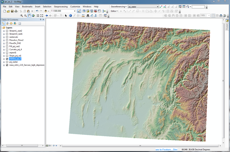
1. Hillshade – Now you are ready to create a Hillshade layer. Adding a Hillshade layer under the topography helps increase the ‘realness’ of the map. Hillshade layers are derived from elevation layers. They calculate surface light and shadow based on a sun position. They are used to create a relief perspective. To do so, click on ArcToolbox in the main navigation bar of your ArcMap project. From there, select Spatial Analyst Tools->Surface->Hillshade. Double-click on Hillshade. In the Hillshade dialog, make sure the Input raster points to your projected DEM file. You could also drag and drop your projected DEM file from Table of Contents into the box under Input raster. Save the output raster in your Arc1_exercise_for_students folder. Do not change the default values for Azimuth and Altitude. Do not check the Model Shadows box. Generally, Hillshade DEMs are clearer if the basic elevation layer is multiplied by 2 or 3. In this case changing the Z factor to 2 will multiply the input DEM by 2 before computing Hillshade. Click OK. The Hillshade raster will be automatically added to ArcMap. Right click on your Hillshade layer and go to Layer Properties-> Display and set Transparency to 30%. Save your .mxd file. It should look something similar to this:

 

Save your Hillshade map by following steps listed under Part 1 (A1-b). You will include this map in your final PDF file.

2. Slope, Aspect, and Curvature – Go to ArcToolbox to calculate Slope, Aspect (slope direction), and Curvature. Use your projected DEM raster as the Input raster. Make sure to save your .mxd file. To learn more about these tools, go to Help in the main navigation bar and select ArcGIS Desktop Help. Use the Search tab to look up information on these tools.

a. Explain what each function (Slope, Aspect, and Curvature) does.

b. Why geoscientists would be interested in the output of these functions? For example, are there geomorphic/surface processes we have discussed in class that depend on these parameters?

To turn in: Save all of your maps (4 of them: Hillshade, Slope, Aspect and Curvature) by following steps listed under Part 1 (A1-b). Make sure each map shows title, legend, scale bar, grids, and your name. You will include these maps as well your answers to 2a-b in your final PDF file.

 

C. Hydrologic Terrain Analysis

In this section, you use the hydrology tools to model the flow of water across your DEM surface. These tools can be applied individually or used in sequence to create a stream network or delineate watersheds. In this exercise, you will use the following tools in the following order: Fill, Flow Direction, Flow Accumulation, Stream Network, Stream Order, Stream Link and stream to Feature.

1. Fill - Go to ArcToolbox->Spatial Analyst Tools->Hydrology. Use the Fill tool to fill the sinks in your elevation grid. If cells with higher elevation surround a cell, the water is trapped in that cell and cannot flow. The Fill function modifies the elevation value to eliminate these problems. Double click on Fill and drag and drop your DEM file into the box under Input surface raster. Select Arc1-exercise_for_students folder as the location of your Output surface raster and give it an appropriate name (e.g., …dem_fill). Click OK. The fill layer will be added to your map. This process may take a few minutes. You do not need to turn in this map.

2. Flow Direction – This function computes the flow direction for a given grid. The values in the cells of the flow direction grid indicate the direction of the steepest descent from that cell. Go to ArcToolbox->Spatial Analyst Tools->Hydrology. Double click on the Flow Direction tool. Drag your Fill file (from section C1) into the box under Input surface raster. Select Arc1_exercise_for_students as the location of your Output surface raster and give it an appropriate name (e.g., …dem_flow_dir). Click OK. The flow direction layer will be added to your map. This process may take a few minutes.

a. Why is flow direction important in hydrologic modeling?

b. In your map, in what color are the cells flowing west displayed?

Save your flow direction map by following steps listed under Part 1 (A1-b). Make sure your map shows title, legend, scale bar, grids, and your name. 

3. Flow Accumulation - This function computes the flow accumulation grid that contains the accumulated number of cells upstream of a cell, for each cell in the input grid. Go to ArcToolbox->Spatial Analyst Tools->Hydrology. Double click on the Flow Accumulation tool. Drag and drop your flow direction (from section C2) into the box under Input surface raster. Select Arc1_exercise_for_students folder as the location of your Output surface raster and give it an appropriate name (e.g., …dem_flow_acc). Click OK. The flow accumulation will be added to your map. This process will take several minutes.

Adjust the Symbology of the flow accumulation layer to visualize high-flow pathways more easily. Change the Symbology method to Classified. Use 2 classes. Click Classify Button and select Manual method. Alter the break value for the first class to 5000. Click OK. Change the Symbology (no color for the first class, black for the second class). Click OK. The cells that are displayed in black have the flow of at least 5000 upstream cells flowing through them. This value is important because it defines the minimum catchment area that the calculation is done on.  If the value is set too low, then the calculation is done on catchments that are too small to care about for understanding geomorphic processes.

Save you flow accumulation map by following steps listed under Part 1 (A1-b). Make sure your map shows title, legend, scale bar, grids, and your name. 

4. Stream Network – To delineate stream networks from your DEM, use the output from the Flow Accumulation tool, and apply a threshold value using either Con or Set Null. To do this, go to ArcToolbox->Spatial Analyst Tools->Map Algebra->Raster Calculator. Use the following expression: Con("FAC" > 100, 1, 0) – Note that FAC is your input flow accumulation raster. This expression creates a raster where the value 1 represents a stream network on a background of NoData, assigned to all cells with more than 100 cells flowing into them. All other cells are assigned NoData. This makes it easier for you to view the stream network. Save the stream network map by following steps listed under Part 1 (A1-b). Make sure your map shows title, legend, scale bar, grids, and your name.

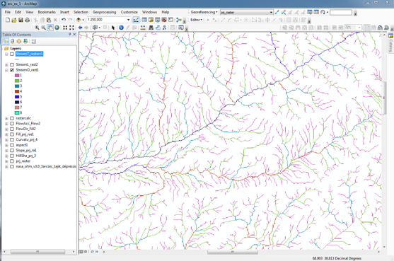
5. Stream Order–Analyze the stream networks from above using the Stream Order function (located in the Hydrology toolbox). When using the Stream Order tool, apply the default Strahler method to assign a numeric order to links in your stream networks. Save your map by following steps listed under Part 1 (A1-b). The Strahler method (also called Strahler order) is a hierarchical scheme for numbering streams. The number assigned to a stream essentially states how large the stream is and how many tributaries are flowing into it. It is a way of comparing streams of similar size. Make sure your map show title, legend, scale bar, grids, and your name. If you zoom in on your DEM, it should look like this:

   

a. Explain what the Stream Order function does and why is its outcome useful.

Note! Save your .mxd file. 

To turn in: Save your maps from Section C by following steps listed under Part 1 (A1-b). Your maps are: Flow Direction, Flow Accumulation, Stream Network, and Stream Order. Make sure each map shows title, legend, scale bar, grids, and your name. Include these maps and your answers to questions asked in this section in your final PDF file. 

 

D. Adding Point Data (e.g. sample locations) to your map

In this section, you learn how to add tabular data that contains geographic locations in the form of x,y coordinates to your map.  You can create a table in Microsoft Excel, create fields, enter values in the fields, save it as a .csv file (Comma Separated Value) or .txt file. To add x,y coordinates to your map, your table must contain at least two fields, one for the x-coordinate and one for the y-coordinate. The values in the fields may represent any coordinate system and units such as latitude and longitude or meters. Now, follow the steps shown below to add three data points that contain information about three hydrologic stations in Tajikistan.

1. Download the hydro_station.csv file to your working folder. Notice the columns: latitude, longitude, station elevation, station name, the start and end dates for operation, and the measurement type. Now that you know what’s inside this file, close it and return to ArcMap. In ArcMap, go to Add Data, navigate to your hydro_station.csv file and add it to Layers. Once the file is added, right-click on it and open it. It should look the same as it was before, except that it is now is inside the ArcMap. Close it, and right-click on it again and go to Display XY Data. The X Field is the Longitude and the Y Field is the Latitude. Leave the Z Field empty. Check the Coordinate System and make sure it is set to: GCS_WGS_1984. Click OK. Turn off all other layers except your projected DEM and Stream Order layers. These maps will be shown underneath the points you just added. Change the Symbology for the points by going to Layer Properties->Symbology and click on the point symbol. Choose a black triangle and increase its size to 18. Click Apply and OK. You can use the Identify icon on the main tool bar  to obtain more information about each point. Click on and move your cursor to one of the points on the map. Click onit to display information (these are the field values you saw earlier). Close the dialog. Now add the station name for each point as text on your map. It is better to do this in Layout View. Go to View->Layout View, then Insert->Text. Include this map in your final PDF file.
2. Indicate the Stream Order for the rivers where the following hydrologic stations are placed:

Nurak:_________, Mahe Now:__________, Panj:___________

To turn in: Save your map from Section D by following steps listed under Part 1 (A1-b). Your map should include the three station points and their names (all shown over your DEM and Stream Order layers). Make sure your map includes title, legend, scale bar, grids, and your name. Include your map and answer to the above question in your final PDF file. 

---

What To Hand In:  

Hand in your answers to questions and all maps from Part 1 as one PDF file (not Word) through the Illias website. Make sure each map shows title, legend, scale bar, grids, and your name. Use section headings (e.g., Part 1, Section A, Question 2a) to indicate what question you are answering. 

• To add files to Word or Libre office document before making the PDF file we suggest you: export and save the relevant maps as tiff files from the ArcMap window (go to File -> Export Map). Then insert the tiff files into a MS Word document and save the document as PDF.
• For each map you put in the PDF file add well written figure caption to the map.  Write the caption as if you were writing it for a scientific paper or business report.  For example, the first sentence of the caption should say in general terms what is plotted. The following sentence should describe how the analysis was done, and what the primary result is that the reader should see in the plot.
• Hand in your final PDF file via the Ilias website.
• No late assignments will be accepted (we’re not kidding).