---

Tutorial 2: How to handle data and create maps.

 

 

OBJECTIVE:

This exercise gives you an overview of data handling and presentation in ArcGIS.

More specifically, in this exercise you will learn:

• To define a coordinate system for your spatial data
• To georeference scanned maps/images
• To digitize, add features and edit attributes of features in ArcMap
• To use an example online fault database for adding fault attributes in ArcMap

You will use the final product of this exercise (i.e., neotectonic map of the Pamir) for Part 3 (final class project) of this exercise to locate suitable sites for new schools to be built by the Central Asia Institute in Tajikistan.  

 

Remember:

• Bring a USB flash drive to class, create a folder and name it ArcGIS_Exercise2. Save all files related to this exercise to your USB drive.
• Set the mxd’s data source to relative paths. See Part 1 of this exercise for instruction.
• Save your ArcMap (.mxd file) regularly.

 

 A. Georeferencing Images

1. Start ArcMAP. Begin with a new, blank document. Right click on Layers shown in the Table of Contents. Open Data Frame Properties and go to Coordinate System tab. Note that no coordinate system has been assigned to your layers. Click OK. Download the zip-file containing the DEM  nasa_srtm_v3.0_3arcsec_pamir.tif.zip, save the file in your working folder and unzip it. Then click on the Add data button and navigate to your folder where your DEM file is. Select and add nasa_srtm_v3.0_3arcsec_pamir.tif . You will be asked if you like to create pyramids. Click Yes.

Move the cursor over the map. Look at the lower right-hand corner of the page. You will see units displayed in decimal degrees. Geographic coordinate systems (GCS) most commonly have units in decimal degrees measuring degrees of longitude (x-coordinates) and degrees of latitude (y-coordinates). Find out what coordinate system your elevation data are in by examining the layer’s properties.

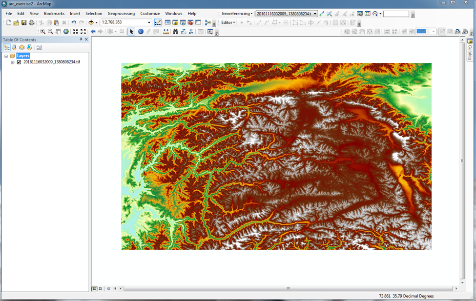
Your DEM is displayed as a gray scale image. Change this setting by choosing a different color ramp to improve the visualization of the terrain. Try picking “Elevation #1” for Color Ramp, and set Type shown under Stretch to Percent Clip. Click Apply. If you are happy with the result, click OK. If not, choose a different setting. Your map may look something like this:

2. Some images such as your DEM file (GeoTIFF) contain georeferencing information in their header file. ArcGIS looks for this information when displaying the image. If there is no information available about the location of your image, you will have to georeferenced it manually. Click on the Add data button and navigate to the ArcGIS 2 exercise folder where your JPEG file is. Select and add pamir_neotectonic_map.jpeg. Notice the warning sign: unknown spatial reference! Click OK. To see the image, right-click on the file name and select Zoom to Layer. You should now see the image. Follow the steps shown below to georeference your image:

• Go to your DEM file. You will use it to georeference your image. Display the DEM file and zoom in to the approximate area that is covered by your image to which this layer will be added. This does not have to be exact as it is done just to provide you with an easier workspace.
• In the Georeferencing toolbar (Customize/Toolbars/Georeferencing), select the layer that corresponds with your image (your JPEG file). Then click on Georeferencing button and select Fit to Display. Your image should be displayed over the DEM layer. To georeference/align your image to the DEM data, you need to find features in your DEM layer that are also visible in the image. These features can be streets, buildings, rivers, or topographic features such as basins, mountain ranges, etc. Take a look at your DEM and image and identify features that can be used to align the two layers. These features will be your ground control points that link locations in the image with locations in the DEM layer. To visualize your image and DEM layers together, go to the Layer Properties for your image, click on Display, and set Transparency to 20%. Click OK.
• From the Georeferencing toolbar, select the Add Control Points icon .

Use your mouse to left click on a known point on the JPEG image. This will place a cross mark on that location. Then, left click on the matching control point in your DEM layer. This will ‘move’ the image and better align the control points. Repeat this step with each control point. It may be a good idea to zoom in on your image when adding control points for increasing accuracy. For every set of control points you create, an entry is created in a table that records the original coordinates, the control point coordinates, and the residual error. Access the table by choosing the View Link Table icon from the Georeferencing toolbar. Entries in this table can be deleted one at a time (highlight the entry in the table and click the delete icon).

• The number of points/links you need to create depends on the method you plan to use to transform the image to map coordinates. However, adding more links will not necessarily yield a better registration. If possible, you should spread out the links over the entire layer rather than concentrating them in one area. Typically, having at least one link near each corner of the image and a few throughout the interior produce the best results. In general, the greater the overlap between the image and your DEM, the better the alignment results since you will have more widely spaced points with which to georeferenced the image. Select at least four links for georeferencing your image.

• After creating your links, you are ready to transform (or warp) the image to DEM layer coordinates. Warping uses a mathematical transformation to determine the correct map coordinate location for each cell in the raster. Use a 1st-order - or affine - transformation to shift, scale, and rotate your image. Straight lines on the image are mapped onto straight lines in the warped raster. Thus squares and rectangles on the raster are commonly changed into parallelograms of arbitrary scaling and angle orientation. A 1st-order transformation will probably handle most of your georeferencing requirements. With the minimum of three links, the mathematical equation used with a 1st-order transformation can exactly map each raster point to the target location. Any more than three links introduces errors, or residuals, that are distributed throughout all the links. In practice, add more than three links. Given only three, if one link is positioned incorrectly, it has a much greater impact on the transformation. Thus, even though the mathematical transformation error may increase as you create more links, the overall accuracy of the transformation will increase as well.

• When you are happy with the georeferencing process, create a new image with the coordinates stored. To do so, go to Georeferencing ->Rectify. Choose an appropriate output location and name for your new image. Click Save.

• Add the new image to your ArcMap project, and uncheck the box next to the old image. Save your .mxd file. Find out what coordinate system your new image is in. In the next section, you will digitize features from your new image into the DEM layer. To do so, you must ensure that your image and DEM layer share the same coordinate system.

 

 B. Digitizing and Adding Data

1. The ArcCatalog lets you create new feature classes and modify them by adding, deleting, and indexing attributes. While you can change the structure and properties of a feature class in ArcCatalog, you must use ArcMap to modify its features and attributes. Load your rectified image. Then open ArcCatalog and navigate to your workspace. Right click: New->Personal Geodatabase. Insert ‘active_faults’ for Right-click on it: New->Feature Class. Type in ‘fault_line” for Name and select Line Features for Type. Click Next. Use the same coordinate system as the one you used for your image in the previous section. Click Next. Keep default values for XY Tolerance, and click Next. Under Field Name, enter the following new fields:

NAME (this is the fault name)

EXPOSURE (this indicates the fault exposure level such as exposed, partially exposed, or concealed)

TYPE (this refers to fault type: normal/reverse/strike-slip/thrust)

GEOL_RATE (this is the geologic slip rate given in mm/yr)

GEOD_RATE (this is the geodetic slip rate given in mm/yr)

EARTHQUAKE (this indicates if there is any historic earthquake associated with the fault: Yes/No)

LITERATURE (this field includes all references for the above information, e.g., Schurr et al., 2014 for your image)

Set all Data Type to ‘Text’ with the exception of slip rates which should be set to ‘Double’. Click Finish. The fault_line feature class will be added to your ArcMap project automatically.

2. In the main navigation bar, click on Editor  and Start Editing:

Then, click on Create Feature and select your feature class ‘fault_line’. Choose Line from Construction Tools. Close the window. In the ArcMap main window, make sure your rectified image (slightly transparent) is show over your DEM layer. The red lines (solid and dashed) on your image represent faults that are likely to be active. Choose one of the red lines on this image for digitization. To begin digitizing a fault trace, click with the mouse and follow the trace of the desired fault. It is a good idea to zoom in on your image when digitizing features. Double-click or hit F2 to finish the trace. Save your edits by going to the Editor toolbar, click on Editor->Save Edits.

3. To edit the attributes of your features (i.e. fault lines), go to your ‘fault_line’ layer in the Table of Contents. Right-click on it and Open Attribute Table. You will see all columns including the ones you created in ArcCatalog. The attributes you created earlier are editable. For example, you can type in ‘strike-slip’, ‘normal’ or ‘reverse’ for TYPE. For EXPOSURE, you can type ‘exposed’ or ‘concealed’. Use the information shown on your georeferenced image and its legend to fill in the appropriate fields in your attribute table. If the information you need is not shown on the image (e.g., slip rates), leave the field blank. We will return to these empty fields later. When you are done, close the Table and save your edits and the .mxd file.

4. To get some practice, repeat steps 2-3 for a few more faults that are likely to be active (i.e., solid and dashed red lines on the image).

5. Now, go to https://esdynamics.geo.uni-tuebingen.de/faults/.This is an online database that allows you to access information on active faults in Central Asia. On the main homepage, you see an interactive map. The red lines mark the location of Quaternary faults that are believed to be active. Now, bring your mouse cursor to the map and use your mouse wheel to zoom in on the country of Tajikistan. You should see something like this:

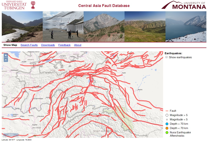
Does this look familiar to you? Click on the fault system to which the black arrow in the above image is pointing. This should take you to an information page specific to this fault system. Use this information to complete the attribute table in your ArcMap project. A few things to keep in mind:

- If you see ‘insufficient data’ shown for slip rate fields in the online database, leave these fields empty in the attribute table in ArcMap. Similarly, if some fields are not shown for some faults in the online database, it means there is insufficient data. Leave these fields empty in the attribute table of your ArcMap project.

- For slip rates that are given in range (e.g., 10-15 mm/yr), take the average value and enter it in the attribute table of your ArcMap project. Save your edits and the .mxd file.

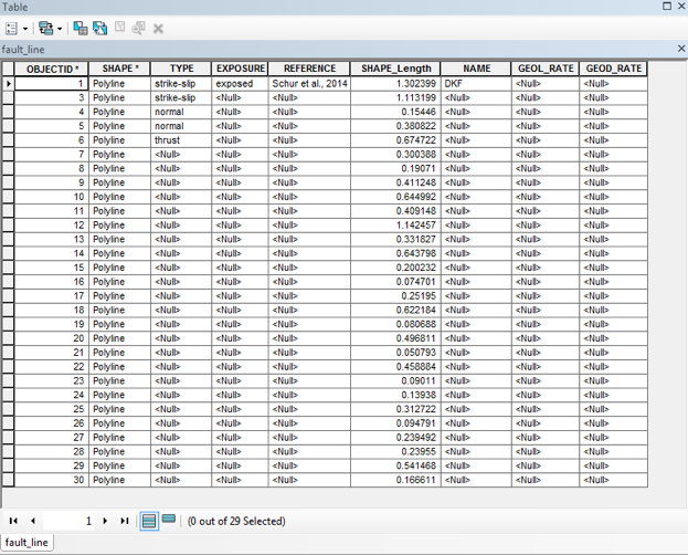
Turn in: Take a screenshot of your completed attribute table and include it in your final PDF file. It should look similar to this (with appropriate values entered in the fields shown as “Null”)”

  

6. Right Click on your fault_line layer and go to Layer Properties. Click on the Symbology tab. Choose ‘Unique values, many’ from Categories in the Show column on the left. Select Type under the Value Fields, and click on Add All Values. You should be able to see different types of faults shown in different symbols. Right click on each symbol to change how it appears. Show all normal faults in red, thrust/reverse fault in black, and strike-slip faults in blue. Increase the line width to 2. Save all your changes. In the Table of Contents, make sure to check the boxes for your DEM and fault_line layers. Uncheck other boxes. You should be able to see you fault lines (color-coded by type) over your elevation map. This is your final map. Make sure it has a title, legend, scale bar, grids, and your name on it.

Turn in: Export your final map as TIFF and include it (with a caption) in your final PDF file.

 

References

Schurr, B., Ratschbacher, L., Sippl, C., Gloaguen, R., Yuan, X., and Mechie J.: Seismotectonics of the Pamir, Tectonics, 33, 1501–1518, 2014.

 

---

What To Hand In:  

Please hand in your final map (with appropriate caption) and a screenshot of your final attribute table from Part 2 as one PDF file (not Word) through the Illias website. Make sure your map shows title, legend, scale bar, grids, caption and your name.

• To add files to Word or Libre office document before making the PDF file we suggest you: export and save your map as a tiff file from the ArcMap window (go to File -> Export Map). Then insert the tiff file into a MS Word document and save the document as PDF.
• Add a well written figure caption to your map. Write the caption as if you were writing it for a scientific paper or business report. For instance, explain what your map shows, cite your data sources, and list other useful information such as the coordinate system for your map.
• Include the final attribute table in the PDF file.
• Hand in your final PDF file via the Ilias website.
• No late assignments will be accepted (we’re not kidding).